Discount Curves

import datetime as dt
import math
import pandas as pd
import matplotlib.pyplot as plt
from rivapy.marketdata.curves import DiscountCurve
from rivapy.enums import DayCounterType, InterpolationType, ExtrapolationType


%load_ext autoreload
%autoreload 2
#the next lin is a jupyter internal command to show the matplotlib graphs within the notebook
%matplotlib inline

Definition of Discount Curves

A discount curve

• stores discount factors for different maturities,

• has an interpolation to compute discount factors for arbitrary maturities,

• has an extrapolation to compute discount factors for arbitrary maturities after the latest given maturity,

• has a day counter to convert dates to year fractions to apply the inter- and extrapolation.

Under the assumption of continuous compounding, the discount factor \(df\) for a cashflow at maturity \(T\) based on a constant discount rate \(r\) is defined as

\[df(T) = e^{-rT}\]

where \(T\) is the time to maturity as year fraction.

Creating Discount Curves

Setup the specification

To setup a discount curve, we need the following information:

Object id

Nearly every structure in the analytics library has an object id. An object id allows for nice logging and exceptions (which object created the message/error) and is also used as identifier for retrieving objects from containers.

object_id = "Test_DC"

Reference date

A reference date is needed for all objects representing market data. Dates entering analytics objects must be analytics ptimes.

Most of the functions provided by market data objects also get a calculation/valuation date and some logic is applied if this date is after the reference date. For a discount curve, if the valuation date is after the reference date, the forward discount factor is returned.

The help function provides information about the function mentioned in its arguments (in parentheses). Uncomment the line to see the information about the analytics.ptime function.

refdate = dt.datetime(2017,1,1,0,0,0)

Dates and corresponding discount factors

We need a list of dates and a list of discount factors. Here, we must use the analytics (C++ swigged) vectors to create the list of dates. We use a helper method which just gets a list of number of days and a reference date and returns the resulting dates from adding the number of days to the reference date. To view the created list of dates, uncomment the 4th and 5th line of the following code.

To calculate the discount factors from a constant rate, we need to provide the constant rate and calculate the discount factors according to the desired compounding frequency.

days_to_maturity =  [1, 180, 365, 720, 3*365, 4*365, 10*365]
dates = [refdate + dt.timedelta(days=i) for i in days_to_maturity]
discount_rate = 0.03
df = [math.exp(-d/365.0*discount_rate) for d in days_to_maturity]

Day count convention

Additionally, we need to provide the discount curve with a day count convention. The different options are provided in the enums module. Here, we apply the ACT365FIXED day count convention where the number of days between two dates is divided by 365. For other examples please refer to the Roll conventions, day counters and schedule generation notebook.

Interpolation type and extrapolation type

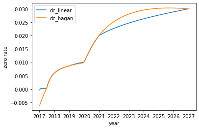
The interpolation is necessary to compute discount factors for arbitrary maturities until the last maturity provided; the extrapolation is necessary to compute discount factors for arbitrary maturities after the last given maturity. Here, we use HAGAN_DF as interpolation type and use no extrapolation. For an overview of interpolation and extrapolation types please refer to the enums module.

The main advantage of the The HAGAN_DF interpolation, also called the monotone convex method (unameliorated version), is that in contrast to the other methods, it ensures forward rates to be positive and is, hence, the probably most suitable interpolation method for financial problems. The method is described in depth in: Hagan, West, “Methods for Constructing a Yield Curve”, 2008.

The following diagrams show the differences between the linear and HAGAN_DF interpolation for a newly created discount curve.

refdate = dt.datetime(2017,1,1,0,0,0)
days_to_maturity =  [1, 180, 365, 720, 3*365, 4*365, 10*365]
rates = [-0.0065, 0.0003, 0.0059, 0.0086, 0.0101, 0.02, 0.03]
dates = [refdate + dt.timedelta(days=i) for i in days_to_maturity]
dsc_fac = [math.exp(-rates[d]*days_to_maturity[d]/365) for d in range(len(rates))]

dc_linear = DiscountCurve('dc_linear', refdate, dates, dsc_fac, InterpolationType.LINEAR,
                          ExtrapolationType.NONE, DayCounterType.Act365Fixed)
dc_hagan = DiscountCurve('dc_hagan', refdate, dates, dsc_fac, InterpolationType.HAGAN_DF,
                        ExtrapolationType.NONE, DayCounterType.Act365Fixed)


dc_linear.plot(discount_factors=False)
dc_hagan.plot(discount_factors=False)
plt.xlabel('year')
plt.ylabel('zero rate')
plt.legend();

Setup the discount curve

Our discount curve is given the name dc and is defined as an analytics.DiscountCurve object which we provide with the information described before.

dc = DiscountCurve(object_id, refdate,dates, df,
                            InterpolationType.HAGAN_DF,
                            ExtrapolationType.NONE,
                             DayCounterType.Act365Fixed)
#help(analytics.DiscountCurve)

Compute Discount Factors

This section is only to manually derive some discount factors from the recently created discount curve.

a. Maturity in 180 days from the reference date

The value function returning a discount factor needs two arguments: the calculation date (here we use the current reference date) and the maturity for which the discount factor shall be computed. Hence, in a first step, the maturity in 180 days has to be converted into a date. Subsequently, the discount factor is computed using the value function. Finally, the print function gives us the computed discount factor of the value function.

df1 = dc.value(refdate, refdate + dt.timedelta(days=180))
print("DF for T=180 days: ", df1)

DF for T=180 days:  0.9853143806656076

b. Forward discount factor for a maturity in 180 days in 90 days

If the valuation date given is in the future, the value function returns the forward discount factor. The following example gives us the forward discount factor for a maturity in 180 days in 90 days.

fwd_df = dc.value(refdate + dt.timedelta(days=90), refdate + dt.timedelta(days=180))
print("Fwd-DF for T=180 days in 90 days: ", fwd_df)

Fwd-DF for T=180 days in 90 days:  0.9926300321180352

A check proves that the result equally the forward discount curve.

df2 = dc.value(refdate, refdate + dt.timedelta(days=90))
print("Fwd-DF (manual calculation): ", df1/df2)

Fwd-DF (manual calculation):  0.9926300321180352

c. Valuation dates before the reference date

Valuation dates before the curves reference date result in an exception (uncomment the following code to see the exception).

#dc.value(refdate + dt.timedelta(days=-90), refdate + dt.timedelta(days=90))

Plotting Discount Curves

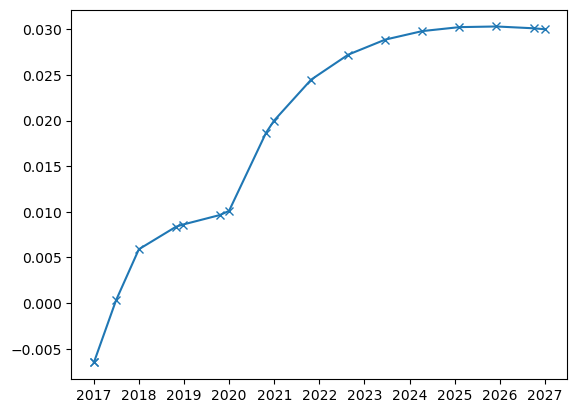
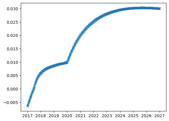
To plot a curve one can simply call the curve’s plot method. This method plots either the discoutn factors or the rates (depending on the argument discount_factors). The granularity of the timegrid on which the curve is plotted can be determined by the argument days. Arguments to matplotlibs plot function can be given using the respective kwargs.

#Example with coarse timegrid
dc_hagan.plot(days=300, marker='x')
#Example with fine timegrid
plt.figure()
dc_hagan.plot(days=10, marker='x')

Exercises

• Create a second discount curve with non-flat rate structure.

• Plot the second discount curve and the first discount curve together in one figure.

• Create a third discount curve exactly as the second but with interpolation LINEARLOG and compare the differences of results using different interpolation schemes (note that finding the correct ensemble of dates and discount factors, forward rates may not be smoothly interpolated with LINEARLOG).

• Write a function computing a simply (continuously) compounded rate for a given discount factor and year fraction.

• Write a function computing an annually compounded rate for a given discount factor and year fraction.

• Find and modify the plot function from above so that the user can additionally choose which compounding rate is used when plotting the rate.

---