Mixing long-term and short-term optimization targets

In energy, we typically face very short-term optimization tasks (e.g. 15min intervals in power) as well as long-term effects such as saisonality. Bringing both together in optimization can easily make complexity explode – if we optimize all assets on the most granular time grid. In our approach we allow all assets bring along their own time-scale, which may be different from the time-scale that is used on portfolio level.

In this example we explain the feature using a rather simple example:

• power market with hourly prices that exhibit an hourly as well as a seasonal structure

• a short-term storage such as a smaller pump storage or a battery that is optimized hourly on a daily basis - but not across more than a week

• a long-term storage such as a high-volume hydro reservoir that is optimized across the whole seaon on a biweekly basis

Some prerequisites

Basics

import numpy as np
import pandas as pd
import datetime as dt
import eaopack as eao
import matplotlib.pyplot as plt

Define portfolio

We use three different assets:

• Market: a simple contract with a given market price

• Short-term storage, acting on an hourly basis. We reduce the complexity by enforcing that the optimization is done for every day, but not across weeks

• Long-term storage acting on a weekly level for the whole season: We reduce complexity by assuming the same (here flat) profile for all hours within two weeks

Note: For sake of clarity in the charts we do the optimization on daily granularity. Finer overall granularity (e.g. hours) is defined on portfolio level in the timegrid

start = dt.date(2021,1,1)
end   = dt.date(2021,12,31)

# the basic setup
node = eao.assets.Node('node')
timegrid = eao.assets.Timegrid(start, end, freq = 'd')
market = eao.assets.SimpleContract(name = 'market', price = 'price', nodes = node ,
                min_cap= -1000., max_cap=1000., start = start, end = end)
# daily flex
st = eao.assets.Storage('ST storage', nodes = node, \
        start=start, end=end, size=10, \
        cap_in=2/24, cap_out=2/24, start_level=5, end_level=5, \
        block_size= 'W')
# weekly flex
lt = eao.assets.Storage('LT storage', nodes = node, \
        start=start, end=end, size=500, \
        cap_in=2/24, cap_out=2/24, start_level=100, end_level=100, \
        freq = '14d')

# price with seasonal and daily pattern
prices ={'price': 10*np.sin(np.linspace(0,2*np.pi, timegrid.T)) \
                + 2*np.sin(np.linspace(0,7*12*np.pi, timegrid.T)) \
                + 2*np.sin(np.linspace(0,7**24*2*np.pi, timegrid.T))}

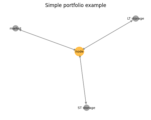
portf = eao.portfolio.Portfolio([market, st, lt])

The below network chart shows the setup of the portfolio.

eao.network_graphs.create_graph(portf = portf, title = 'Simple portfolio example')

Perform the optimization

op    = portf.setup_optim_problem(prices, timegrid)
res = op.optimize()
out = eao.io.extract_output(portf, op, res, prices)

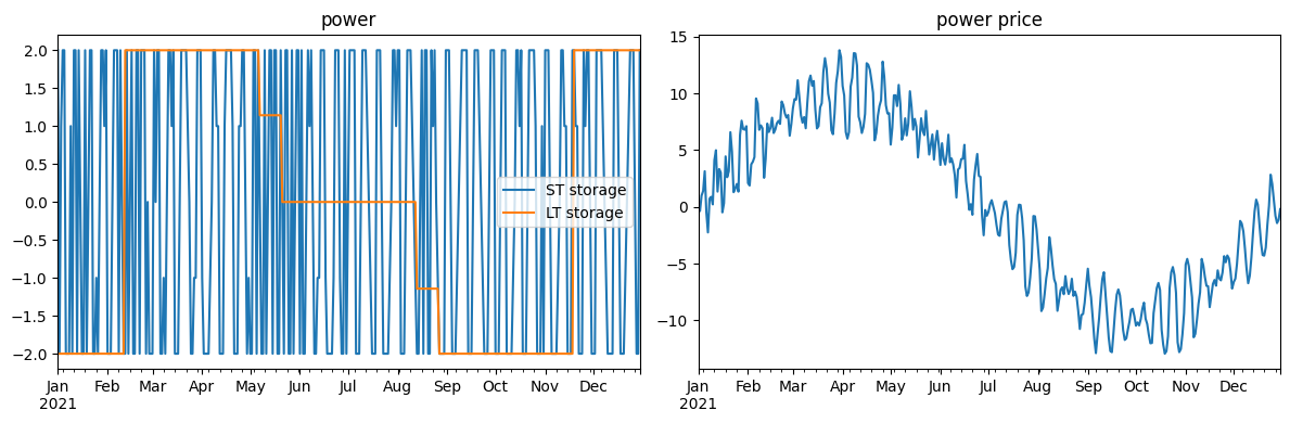
Create charts and interpret the results

fig, ax = plt.subplots(1,2, tight_layout = True, figsize=(12,4))
out['dispatch'][['ST storage', 'LT storage']].plot(ax = ax[0], style = '-')
out['prices']['input data: price'].plot(ax = ax[1], style = '-')
ax[0].set_title('power')
ax[1].set_title('power price')
plt.show()