Combined Heat and Power
The CHPAsset class represents an asset that can generate both heat and power at the same time and models starting procedures, minimum loads, ramping and a minimum runtime.
Technical Details
Input Parameters
Possible input parameters of the CHPAsset are
Ramp \(r\)
Conversion efficiency \(\alpha\) from heat to power.
Maximum share heat \(\beta\)
Minimum capacity \(l_t\) for every timestep \(t \in \left\{0,\dots, T-1\right\}\)
Maximum capacity \(u_t\) for every timestep \(t \in \left\{0,\dots, T-1\right\}\)
Dispatch power \(x_{-1}\) from the previous timestep
Dispatch heat \(w_{-1}\) from the previous timestep
Number \(k_{on}\) of timesteps the asset has already been running
Number \(k_{off}\) of timesteps the asset has already been of
Minimum runtime \(m_{run}\)
Minimum downtime \(m_{down}\)
Start ramp specification:
Minimum capacity \(l^{start}_i\) for timestep \(i \in \left\{0,\dots, k_{start}\right\}\) after starting
Maximum capacity \(u^{start}_i\) for timestep \(i \in \left\{0,\dots, k_{start}\right\}\) after starting
Shutdown ramp specification:
Minimum capacity \(l^{shutdown}_i\) for timestep \(i \in \left\{0,\dots, k_{shutdown}\right\}\) before shutting off
Maximum capacity \(u^{shutdown}_i\) for timestep \(i \in \left\{0,\dots, k_{shutdown}\right\}\) before shutting off
Output variables
The following variables are computed for a CHPAsset that runs for \(T\) timesteps:
Dispatch power \(x_t \in \mathbb{R}\), for every timestep \(t \in \left\{0,\dots, T-1\right\}\)
Dispatch heat \(w_t \in \mathbb{R}\), for every timestep \(t \in \left\{0,\dots, T-1\right\}\)
“On”-variable \(a_t \in \left\{0,1\right\}\), for every timestep \(t \in \left\{0,\dots, T-1\right\}\)
“Start”-variable \(s_t \in \left\{0,1\right\}\), for every timestep \(t \in \left\{0,\dots, T-1\right\}\)
“Shutdown”-variable \(d_t \in \left\{0,1\right\}\), for every timestep \(t \in \left\{0,\dots, T-1\right\}\)
When they are not needed to enforce a minimum runtime, start costs or similar, the “on” and “start” variables are removed.
Variable bounds
The output variables are within the following bounds in every timestep \(t \in \left\{0,\dots, T-1\right\}\):
\(0 \leq x_t \leq u_t\)
\(0 \leq w_t \leq \beta u_t\)
\(0 \leq a_t \leq 1\)
\(0 \leq s_t \leq 1\)
\(0 \leq d_t \leq 1\)
Constraints
The following constraints are used in the asset
Minimum and maximum capacity: The virtual dispatch \(\tilde{x}_t = x_t + \alpha w_t\) is 0 when \(a_t = 0\), i.e. the asset is “off”, it is bounded by the start or shutdown specifications during the start and shutdown, and otherwise it is between minimum and maximum capacity, i.e. \begin{align*} \tilde{x}_t &\geq& l_t \left[ a_t - \sum_{i=0}^{k_{shutdown}-1}d_{t+i+1} - \sum_{i=0}^{k_{start}-1}s_{t-i} \right] + \sum_{i=0}^{k_{start}-1}l^{start}_i s_{t-i} + \sum_{i=0}^{k_{shutdown}-1}l^{shutdown}_i d_{t+i+1} \\ \tilde{x}_t &\leq& u_t \left[ a_t - \sum_{i=0}^{k_{shutdown}-1}d_{t+i+1} - \sum_{i=0}^{k_{start}-1}s_{t-i} \right] + \sum_{i=0}^{k_{start}-1}u^{start}_i s_{t-i} + \sum_{i=0}^{k_{shutdown}-1}u^{shutdown}_i d_{t+i+1} \end{align*} for \(t \in \left\{0,\dots, T-1\right\}\). It should be noted that the term \(\sum_{i=0}^{k_{start}-1}s_{t-i}\) is 1 if timestep \(t\) is part of the start ramp and 0 otherwise. Analogously, \(\sum_{i=0}^{k_{shutdown}-1}d_{t+i+1}\) is 1 if timestep \(t\) is part of the shutdown ramp and 0 otherwise. If \(k_{on} > 0\) and \(k_{on}<k_{start}\), i.e. the asset is in the starting process at timestep \(0\), the first \(k_{start}-k_{on}\) timesteps are instead bounded by \begin{align*} l^{start}_{k_{on}+i} \leq \tilde{x}_i \leq u^{start}_{k_{on}+i} \end{align*} for every \(i \in \left\{0, \dots, k_{start}-k_{on}-1\right\}\).
- Ramp: Ensure that the increase/decrease of the virtual dispatch \(\tilde{x}_t = x_t + \alpha w_t\) is bounded by \(r\), unless during timesteps that belong to the start or shutdown ramp, i.e.\begin{align*} \tilde{x}_t-\tilde{x}_{t-1} &\geq& -r \left[ a_{t-1} - \sum_{i=0}^{k_{shutdown}-1}d_{t+i} \right] - u_{t-1}\sum_{i=0}^{k_{shutdown}-1}d_{t+i} \\ \tilde{x}_t-\tilde{x}_{t-1} &\leq& r \left[ a_{t} - \sum_{i=0}^{k_{start}-1}s_{t-i} \right] + u_{t}\sum_{i=0}^{k_{start}-1}s_{t-i} , \end{align*} for \(t \in \left\{0,\dots, T-1\right\}\).
Start constraints: (Only applicable when there is no start- or shutdown ramp specification, otherwise the start variables are defined simultaneously with the shutdown variables, see “start and shutdown constraints”) When the “on” variable changes from “off” to “on”, the start variable has to be 1, i.e. \begin{align*}s_t \geq a_t - a_{t-1},\end{align*} for \(t \in \left\{1,\dots, T-1\right\}\). If \(k_{on} = 0\), i.e. previous state \(a_{-1}\) is “off”, we need the additional condition \begin{align*}s_0 \geq a_0.\end{align*}
Start and shutdown constraints: (Only applicable when start or shutdown ramp are defined) Ensure that the start and shutdown variables are set correctly, i.e \begin{align*} s_t - d_t &=& a_t - a_{t-1} \\ s_t + d_t &\leq& 1 \end{align*} for \(t \in \left\{0,\dots, T-1\right\}\).
Minimum runtime: Ensure that the asset follows the minimum runtime \(m_{run}\) and is on during the start and shutdown ramp, i.e. \begin{align*}a_t \geq s_{t-i}\end{align*} for \(t \in \left\{1,\dots, T-1\right\}\) and \(i \in \left\{1, \dots, m_{run}+k_{start}+k_{shutdown}-1\right\}\). If \(k_{on}>0\) and \(m_{run}+k_{start}+k_{shutdown} > k_{on}\), we need the additional condition \begin{align*}a_i \geq 1,\end{align*} for all \(i \in \left\{0, \dots, m_{run}+k_{start}+k_{shutdown} -k_{on}-1\right\}\).
Minimum downtime: If the asset turns off, it has to stay off for the minimum downtime \(m_{down}\), i.e. \begin{align*}a_t \leq 1 - a_{t-i-1} + a_{t-i}\end{align*} for \(t \in \left\{1,\dots, T-1\right\}\) and \(i \in \left\{1, \dots, m_{down}-1\right\}\). If \(k_{off}>0\) and \(m_{down} > k_{off}\), we need the additional condition \begin{align*}a_i \leq 0,\end{align*} for all \(i \in \left\{0, \dots, m_{down} -k_{off}-1\right\}\).
Maximum share heat: Bound the heat dispatch by a percentage of the power dispatch, i.e. \begin{align*}w_t \leq \beta x_t,\end{align*} for \(t \in \left\{0, \dots, T-1\right\}\).
Example Portfolio
Imports
[ ]:
import numpy as np
import datetime as dt
import matplotlib.pyplot as plt
import eaopack as eao
from eaopack.portfolio import Portfolio
from eaopack.basic_classes import Timegrid
from eaopack.optimization import Results
Defining a portfolio
[2]:
node_power = eao.assets.Node('node_power')
node_heat = eao.assets.Node('node_heat')
node_gas = eao.assets.Node('node_gas')
timegrid = eao.assets.Timegrid(dt.date(2021, 1, 1), dt.date(2021, 1, 2), freq='15min', main_time_unit='h')
simple_contract_power = eao.assets.SimpleContract(name='SC_power', price='price_power', nodes=node_power,
min_cap=-30., max_cap=20)
simple_contract_heat = eao.assets.SimpleContract(name='SC_heat', price='price_heat', nodes=node_heat,
min_cap=-30., max_cap=20.)
simple_contract_gas = eao.assets.SimpleContract(name='SC_gas', price='price_gas', nodes=node_gas,
min_cap=-30., max_cap=20.)
chpasset = eao.assets.CHPAsset(name='CHP',
nodes=[node_power, node_heat, node_gas],
min_cap=5.,
max_cap=30.,
extra_costs=0,
conversion_factor_power_heat=0.5,
max_share_heat=0.5,
ramp=10,
start_ramp_lower_bounds=[1, 2],
shutdown_ramp_lower_bounds=[2, 3],
ramp_freq="15min",
start_costs=0.,
running_costs=0.,
min_runtime=0.,
time_already_running=0.,
min_downtime=0.,
time_already_off=1.,
last_dispatch=0.,
start_fuel=0)
prices = {'price_power': np.sin(0.5*np.pi * np.arange(timegrid.T)*np.pi/10)+2,
'price_heat': np.cos(0.5*np.pi * np.arange(timegrid.T)*np.pi/10)+2,
'price_gas': np.ones(timegrid.T)*2,
}
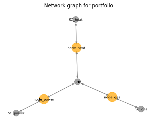
portfolio = eao.portfolio.Portfolio([chpasset, simple_contract_power, simple_contract_heat, simple_contract_gas])
eao.network_graphs.create_graph(portf = portfolio)
Performing the Optimization
[3]:
op = portfolio.setup_optim_problem(prices, timegrid)
res = op.optimize(solver="GLPK_MI")
# res = op.optimize(solver="GLPK", make_soft_problem=True)  # Relax bool variables, i.e. allow "half on"
out = eao.io.extract_output(portfolio, op, res, prices)
out['summary']
[3]:
| Values | |
|---|---|
| Parameter | |
| status | successful |
| value | 238.013408 |
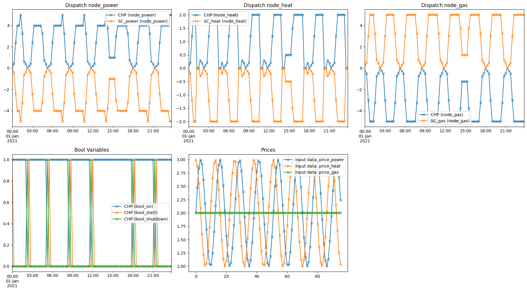
Plotting the Results
[4]:
# Define the grid size to display the figures:
num_imgs_per_row = 3
num_nodes = len(portfolio.nodes)
num_img_rows=int(np.ceil((num_nodes+2)/num_imgs_per_row))
fig, ax = plt.subplots(num_img_rows, num_imgs_per_row, tight_layout = True, figsize=(18,5*num_img_rows))
ax = ax.reshape(-1)

# Plot the dispatch for each node:
current_ax=0
dispatch_per_node = {node: [] for node in portfolio.nodes}
for mycol in out['dispatch'].columns.values:
    for node in dispatch_per_node:
        if '(' + node + ')' in mycol:
            dispatch_per_node[node].append(mycol)
for node in dispatch_per_node:
    out['dispatch'][dispatch_per_node[node]].plot(ax=ax[current_ax], style='-x')
    ax[current_ax].set_title("Dispatch " + node)
    current_ax+=1

# Plot internal variables:
for v in out['internal_variables']:
    out['internal_variables'][v].plot(ax=ax[current_ax], style='-x', label=v)
if out['internal_variables'].shape[1] == 0:
    ax[current_ax].text(0.4, 0.5, "No bool variables present")
ax[current_ax].set_title('Bool Variables')
ax[current_ax].legend()
current_ax+=1

# Plot prices
for key in out['prices']:
    out['prices'][key].plot(ax=ax[current_ax], style='-x', label=key)
ax[current_ax].set_title('Prices')
ax[current_ax].legend()

# Remove empty axes:
for i in range(current_ax+1, len(ax)):
    fig.delaxes(ax[i])
[ ]: